Create animations with MoviePy

If well it is true that one image says more than one-thousand words, an animation can says a full story. For this reason, I have been including animations in all my outreach and scientific talks, going from planets moving in a simulated sky to a curve dancing through data to the rhythm of Gaussian Processes.

Recently, I found MoviePy, a Python library that can help us to create such animations. MoviePy is a library that allows performing video editing. I will not focus on all of its particularities, but on the one that helps us to create animations (gifs or mp4) from a set of png images.

In this post, I show a tutorial on how to create a sequence of png images, and how to use MoviePy to combine them in an animation. If you are only interested in the magic commands to create the animation inside python, go directly here. You can also find a jupyter notebook version of this tutorial here.

Creating a sequence of png images

Let us say that we want to animate some RV model passing through RV data. In this example, we will create the data that we will animate, but keep in mind that in real life, these data would come from our favourite spectrograph and our RV model from some fancy data analysis.

First, let us create a function to compute the RV curve of a planet in a circular orbit

#Load libraries
import numpy as np
import matplotlib.pyplot as plt

#Let us write a function to compute RV for a circular orbit
#input parameters are time t (vector with N elements)
#and the model parameters
#in this case
#params[0] -> vz -> Systemic velocity of the star
#params[1] -> K  -> Doppler semi-amplitude
#params[2] -> P  -> Orbital period
#params[3] -> T0 -> time of minimum conjunction 
#This function returns a vector (N elements) of RVs at the times t
def calcula_RV(t,params):
    vz = params[0]
    K  = params[1]
    P  = params[2]
    t0 = params[3]
    vr = vz - K * np.sin(2*np.pi*(t-t0)/P)
    return vr

Now it is time to give some values to the variables (the values that I use are random, feel free to change it to match your favourite RV exoplanet)

#let us create a time vector between 0 and 10 days with a point each 0.1 days
t = np.arange(0,10,0.1)
#Let us give some values for the 4 parameters that define the RV of a circular orbit
vz = 40 #km/s
K = 0.05#km/s
P = 2   #days
t0 = 13 #days

#Let us call the function to estimate the RV for a circular orbit
rv = calcula_RV(t,[vz,K,P,t0])

Now we can create some simulated data by adding some white noise to the previously computed RVs

#Let us create an error bar of 5 m/s
rv_err = 5e-3
#Create RV data
rv_data = np.random.normal(rv,rv_err)
#Let us plot the model and the data together
plt.plot(t,rv)
plt.plot(t,rv_data,'o')

you should have a plot similar to this one

At this point, we have two arrays: rv_data that contains some simulated data points, and rv that contains the model used to create data. We are now ready to create our animation, we want to plot our data and show how the model is appearing slowly following the data.

First, let us create a routine to create a generic plot with model and data

#Let us create a function to create a plot
#tmodel -> time-stamps of the model
#model  -> model values corresponding to tmodel
#tdata  -> time-stamps of the data
#data   -> model values corresponding to tdata
#fname  -> name of the output file
def plot_data(tmodel,model,tdata,data,fname):
    #This is exactly a matplotlib plotting routine 
    plt.figure(1,figsize=(8,4))
    plt.xlabel('Time (days)')
    plt.ylabel('RV (km/s)')
    plt.plot(tmodel,model)
    plt.plot(tdata,data,'o')
    plt.savefig(fname,dpi=150,bbox_inches='tight')

We can call the plot_data routine inside a for-cycle where we can modify the model to plot at each iteration, in such a way that each new image will show an increasing section of the model. Such for-cycle would look like this

#create a cycle that creates our plots
#In this case, each plot will show all the data and the model will appear one step each time
for i in range(len(t)):
    #Create the filename automatically
    fname = 'rv_'+str(i).zfill(5)+'.png'
    #Create the plot, note how each iteration we plot the first i elements of the model
    plot_data(t[:i],rv[:i],t,rv_data,fname)
    plt.close()

The previous for-cycle will create a series of png images named 'rv_000XX.png', where XX goes from 0 to 99. I would encourage to use ascending numbers similar to this since this will help to identify the correct sequence of the images as shown below.

Creating your animation

At this point, you should be in a directory with a bunch of png images that you want to use to create an animation. Rather the images created using this tutorial or your own png images.

To create our animation we use just a few lines of code

#Load libraries
import glob
import moviepy.editor as mpy

#name of the animation
gif_name = 'rv_animation'

#frames per second
fps = 24

#Create a sorted list with all the png files in our directory
file_list = sorted(glob.glob('*.png')) 

#Create a clip instance using ImageSequenceClip included in moviepy
clip = mpy.ImageSequenceClip(file_list, fps=fps)

#No we can write the animation as a a gif
clip.write_gif(gif_name+'.gif')

You should see some progress bar and after that a message saying that your gif animation is ready. You can also change the last line to create an mp4 file

#No we can write the animation as a a mp4
clip.write_videofile(gif_name+'.mp4')

You should have an animation like the one below

Of course, this is just a basic example, but you can use it to create some other animations, such as:

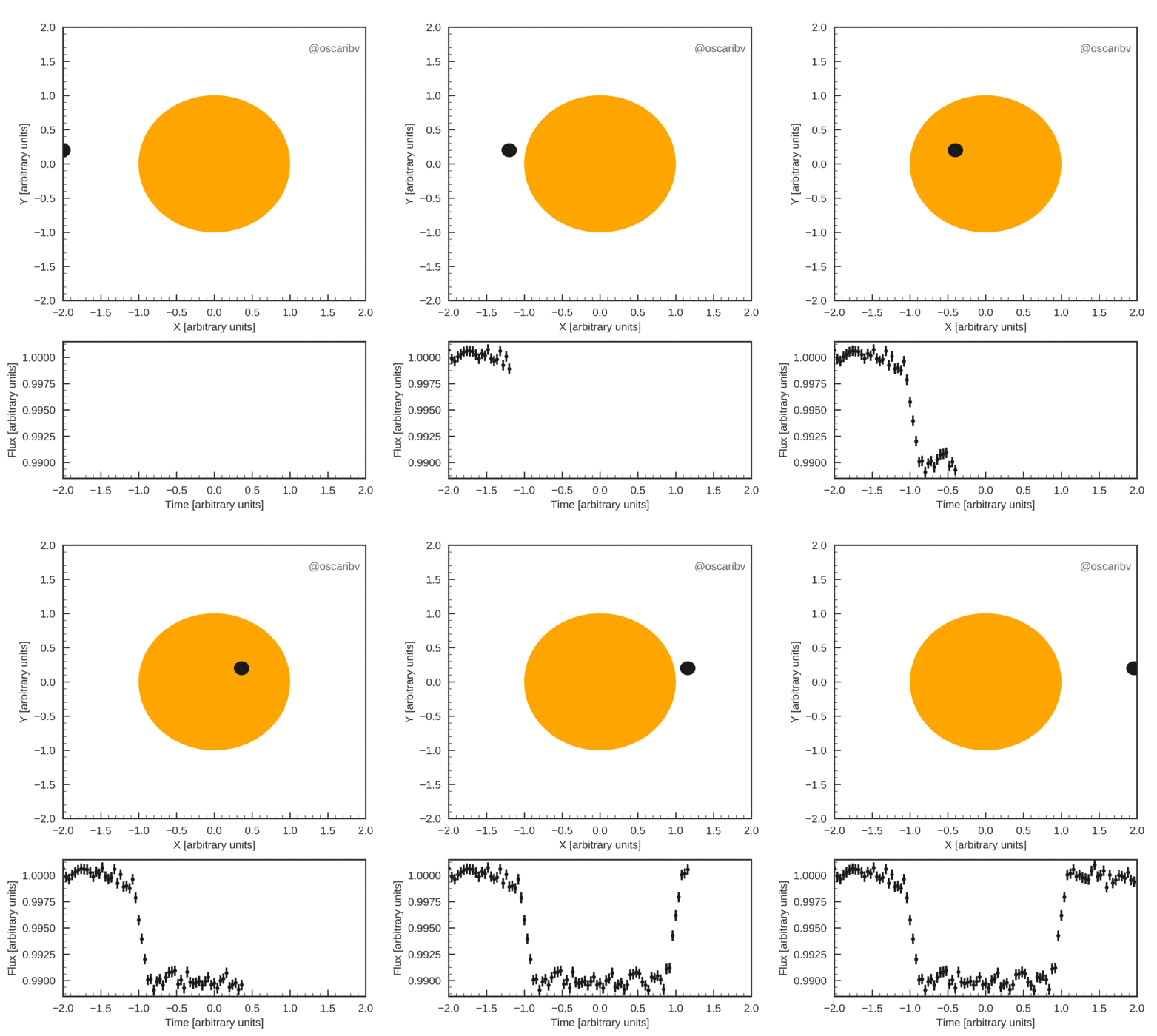
Planets transiting a star

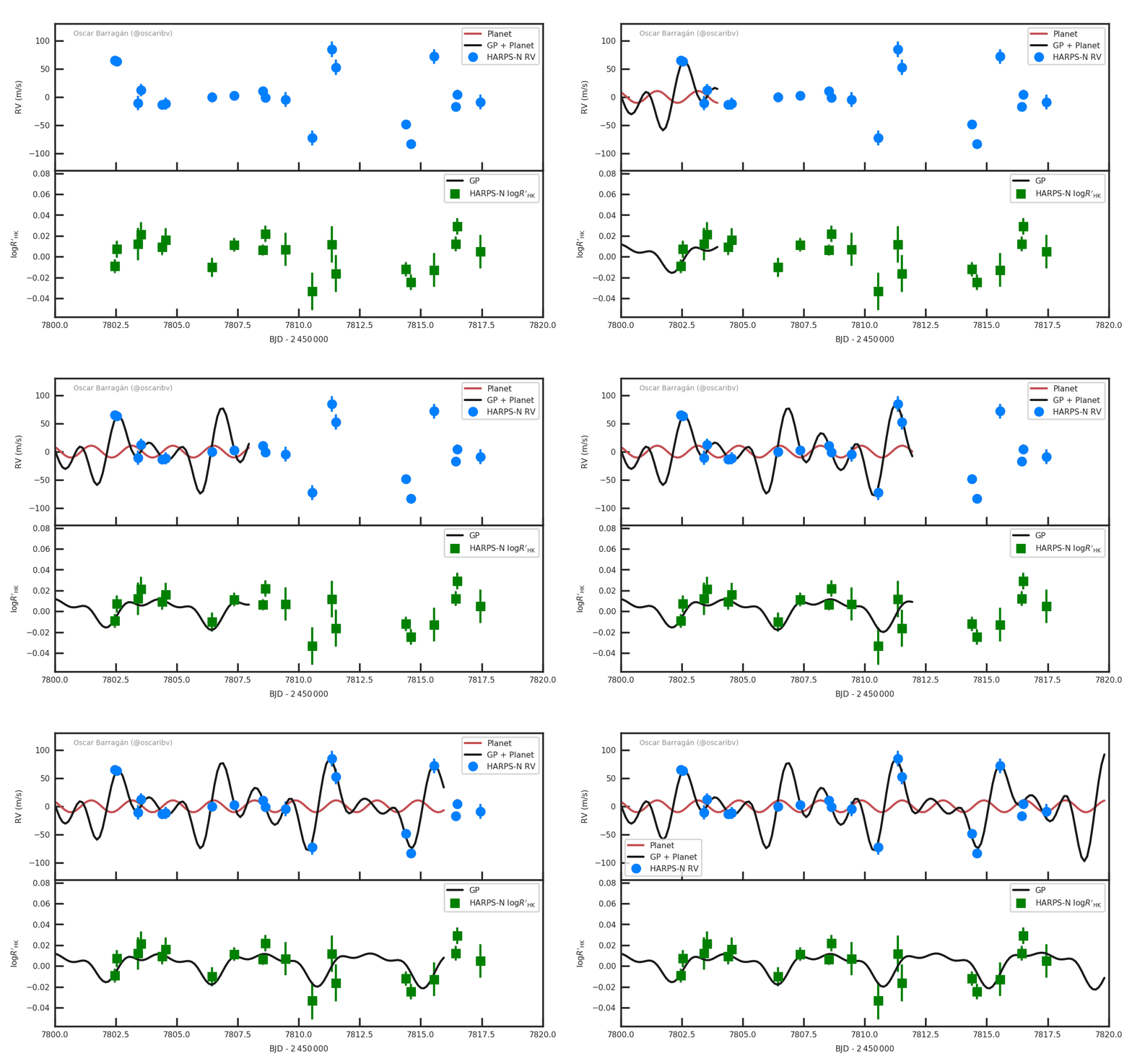
or, as mentioned in the introduction of this post, curves dancing through data to the rhythm of Gaussian Processes

and so on, now the limit is your imagination! I hope you find this post useful to animate data to explain a Universe that is intrinsically dynamic.

This blog post was first posted in https://splox.net/resources/create-animations-with-moviepy/